When we simplify the vocal-tract configuration, we end up with a so-called “three-tube model,” where three uniform tubes are connected to each other. The following is a schematic representation of the midsaggital cross-section:
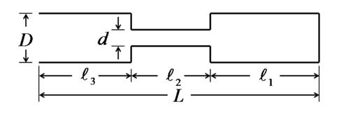
In this figure, the glottis end is on the right, and the lip end is on the left. The first tube is the right one, with length $l_{1}$ and diameter $D$. The second tube is the middle one, with length $l_{2}$ and diameter d. The third tube is the leftmost one, with length $l_{3}$ and diameter $D$. The total length of the three tubes is $L (= l_{1} + l_{2} + l_{3} )$.
If the diameter $d$ of the second tube is small enough compared to the diameter of the rest, that is, $D$, we can assume the tubes are acoustically decoupled and the resonance phenomena in the tubes can be treated independently. In this case, we can think of three resonances of the tubes in lower frequencies. The first resonance is from the first tube. With this tube, both ends are considered to be closed, and the approximation of its first resonance frequency is given by $c / ( 2l_{1} )$. The second resonance is from the third tube. With this tube, one end is open but the other end is considered to be closed, and the approximation of its first resonance frequency is given by $c / ( 4l_{3})$. The third resonance is a Helmholtz resonance from a resonator formed by the first and second tubes. The resonance frequency is given by
$$\frac{ c }{ 2 \pi } \sqrt{ \frac{ A_{2} }{ A l_{1} l_{2} }}$$
where $A$ and $A_{2}$ are the areas of circles with diameters $D$ and $d$, respectively:
$$A = (\pi / 4)D^2 \ and \ A_{2} = (\pi / 4)d^2$$.
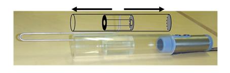
With this three-tube model, a wide range of vowels can be produced by appropriately defining such parameters. To confirm this, let’s take a look at the so-called “sliding three-tube model.” In this model, there is an outer tube, with an inner diameter $D$, and an inner tube, with a hole having the diameter $d$. Because the inner tube slides back and forth inside the outer tube, the location of the constriction can change arbitrarily (see the following photograph).
Now, let’s use the values in the following figure and draw resonance curves as well as plot the measured spectral peak frequencies from actual models. The three resonance curves in this figure are obtained by the three formulas above by simple approximation. (The end correction of 0.82 r with a flange, where r is the radius of the third tube was applied at open end to the Helmholtz resonator, in this figure.)
The dots are the measured peak frequencies, which correspond to the resonances. These spectral peaks are named “formants,” and they are numbered from the lowest frequency: the 1st formant (F1), the 2nd formant (F2), and so on.
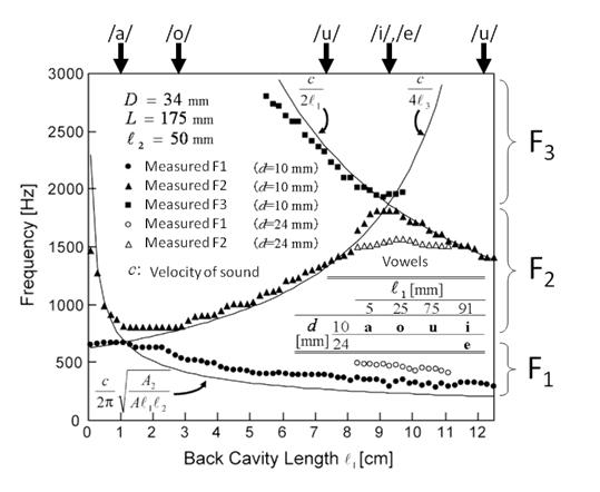
Please note that the horizontal axis is of this figure is the length of the first tube, or $l_{1}$, and the vertical axis is frequency. The short $l_{1}$ is on the left of this figure, and this corresponds to when the constriction is located at the lip end. On the other hand, the long $l_{1}$ is on the right, and this corresponds to when the constriction is located at the glottis end.
From this plot, we can see that vowels /a/ and /o/ are produced when the constriction is in the back, the vowel /u/ is produced when the constriction is in the middle, and the vowel /i/ is produced when the constriction is in the front. The vowel /e/ is produced when the constriction is located at the same position as the vowel /i/, but the diameter of the constriction $d$ is larger.
- Arai, T., “Sliding three-tube model as a simple educational tool for vowel production,” Acoust. Sci. Tech., 27(6), 384-388, 2006.
- Arai, T., “Education in acoustics and speech science using vocal-tract models,” J. Acoust. Soc. Am., 131(3), Pt. 2, 2444-2454, 2012.
- Fant, G., Acoustic Theory of Speech Production, (Mouton, The Hague, Netherlands), pp. 15-90, 1960.